Plotting Examples
The examples below show how wrf-python can be used to make plots with matplotlib (with basemap and cartopy) and PyNGL. None of these examples make use of xarray’s builtin plotting functions, since additional work is most likely needed to extend xarray in order to work correctly. This is planned for a future release.
A subset of the wrfout file used in these examples can be downloaded here.
Matplotlib With Cartopy
Cartopy is becoming the main tool for base mapping with matplotlib, but you should be aware of a few shortcomings when working with WRF data.
The builtin transformations of coordinates when calling the contouring functions do not work correctly with the rotated pole projection. The transform_points method needs to be called manually on the latitude and longitude arrays.
The rotated pole projection requires the x and y limits to be set manually using set_xlim and set_ylim.
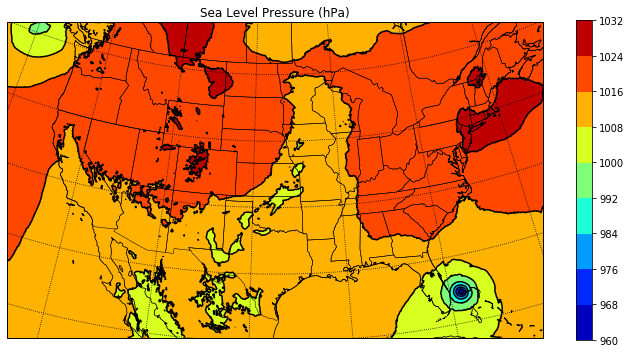
Plotting a Two-dimensional Field
from netCDF4 import Dataset
import matplotlib.pyplot as plt
from matplotlib.cm import get_cmap
import cartopy.crs as crs
from cartopy.feature import NaturalEarthFeature

from wrf import (to_np, getvar, smooth2d, get_cartopy, cartopy_xlim,
                 cartopy_ylim, latlon_coords)

# Open the NetCDF file
ncfile = Dataset("wrfout_d01_2016-10-07_00_00_00")

# Get the sea level pressure
slp = getvar(ncfile, "slp")

# Smooth the sea level pressure since it tends to be noisy near the
# mountains
smooth_slp = smooth2d(slp, 3, cenweight=4)

# Get the latitude and longitude points
lats, lons = latlon_coords(slp)

# Get the cartopy mapping object
cart_proj = get_cartopy(slp)

# Create a figure
fig = plt.figure(figsize=(12,6))
# Set the GeoAxes to the projection used by WRF
ax = plt.axes(projection=cart_proj)

# Download and add the states and coastlines
states = NaturalEarthFeature(category="cultural", scale="50m",
                             facecolor="none",
                             name="admin_1_states_provinces_shp")
ax.add_feature(states, linewidth=.5, edgecolor="black")
ax.coastlines('50m', linewidth=0.8)

# Make the contour outlines and filled contours for the smoothed sea level
# pressure.
plt.contour(to_np(lons), to_np(lats), to_np(smooth_slp), 10, colors="black",
            transform=crs.PlateCarree())
plt.contourf(to_np(lons), to_np(lats), to_np(smooth_slp), 10,
             transform=crs.PlateCarree(),
             cmap=get_cmap("jet"))

# Add a color bar
plt.colorbar(ax=ax, shrink=.98)

# Set the map bounds
ax.set_xlim(cartopy_xlim(smooth_slp))
ax.set_ylim(cartopy_ylim(smooth_slp))

# Add the gridlines
gl = ax.gridlines(draw_labels=True, color="black", linestyle="dotted")
gl.right_labels = False
gl.x_inline = False
gl.top_labels = False

plt.title("Sea Level Pressure (hPa)")

plt.show()
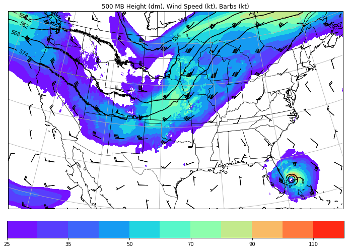
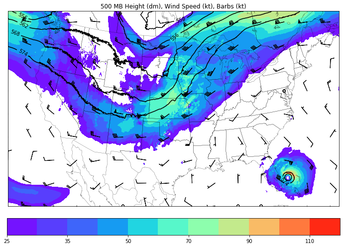
Horizontal Interpolation to a Pressure Level
from netCDF4 import Dataset
import numpy as np
import matplotlib.pyplot as plt
from matplotlib.cm import get_cmap
import cartopy.crs as crs
from cartopy.feature import NaturalEarthFeature

from wrf import (getvar, interplevel, to_np, latlon_coords, get_cartopy,
                 cartopy_xlim, cartopy_ylim)

# Open the NetCDF file
ncfile = Dataset("wrfout_d01_2016-10-07_00_00_00")

# Extract the pressure, geopotential height, and wind variables
p = getvar(ncfile, "pressure")
z = getvar(ncfile, "z", units="dm")
ua = getvar(ncfile, "ua", units="kt")
va = getvar(ncfile, "va", units="kt")
wspd = getvar(ncfile, "wspd_wdir", units="kts")[0,:]

# Interpolate geopotential height, u, and v winds to 500 hPa
ht_500 = interplevel(z, p, 500)
u_500 = interplevel(ua, p, 500)
v_500 = interplevel(va, p, 500)
wspd_500 = interplevel(wspd, p, 500)

# Get the lat/lon coordinates
lats, lons = latlon_coords(ht_500)

# Get the map projection information
cart_proj = get_cartopy(ht_500)

# Create the figure
fig = plt.figure(figsize=(12,9))
ax = plt.axes(projection=cart_proj)

# Download and add the states and coastlines
states = NaturalEarthFeature(category="cultural", scale="50m",
                             facecolor="none",
                             name="admin_1_states_provinces_shp")
ax.add_feature(states, linewidth=0.5, edgecolor="black")
ax.coastlines('50m', linewidth=0.8)

# Add the 500 hPa geopotential height contours
levels = np.arange(520., 580., 6.)
contours = plt.contour(to_np(lons), to_np(lats), to_np(ht_500),
                       levels=levels, colors="black",
                       transform=crs.PlateCarree())
plt.clabel(contours, inline=1, fontsize=10, fmt="%i")

# Add the wind speed contours
levels = [25, 30, 35, 40, 50, 60, 70, 80, 90, 100, 110, 120]
wspd_contours = plt.contourf(to_np(lons), to_np(lats), to_np(wspd_500),
                             levels=levels,
                             cmap=get_cmap("rainbow"),
                             transform=crs.PlateCarree())
plt.colorbar(wspd_contours, ax=ax, orientation="horizontal", pad=.05)

# Add the 500 hPa wind barbs, only plotting every 125th data point.
plt.barbs(to_np(lons[::125,::125]), to_np(lats[::125,::125]),
          to_np(u_500[::125, ::125]), to_np(v_500[::125, ::125]),
          transform=crs.PlateCarree(), length=6)

# Set the map bounds
ax.set_xlim(cartopy_xlim(ht_500))
ax.set_ylim(cartopy_ylim(ht_500))

ax.gridlines()

plt.title("500 MB Height (dm), Wind Speed (kt), Barbs (kt)")

plt.show()
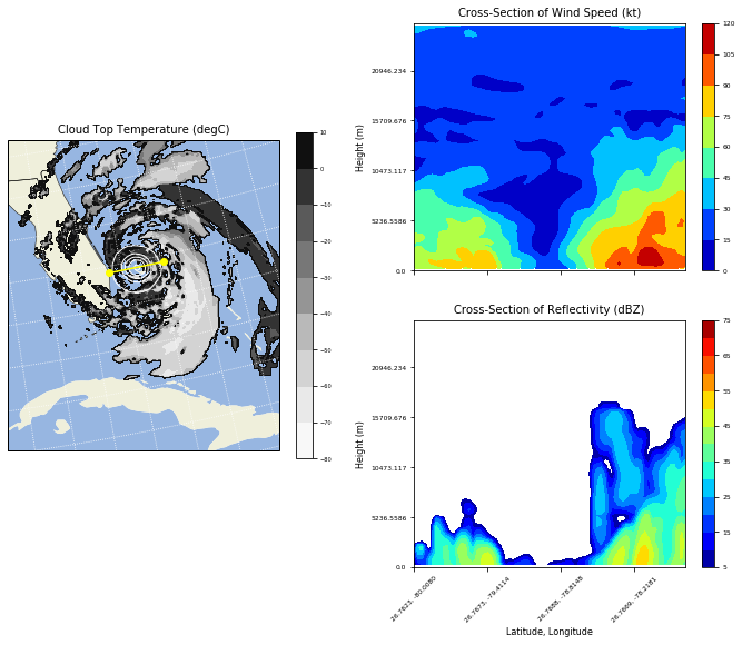
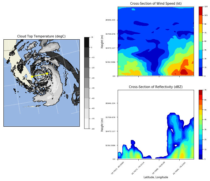
Panel Plots From Front Page
This lengthy example shows how to make the panel plots on the first page of the documentation. For a simpler example of how to make a cross section plot, see Vertical Cross Section.
import numpy as np
import matplotlib.pyplot as plt
from matplotlib.cm import get_cmap
import cartopy.crs as crs
import cartopy.feature as cfeature
from netCDF4 import Dataset

from wrf import (getvar, to_np, vertcross, smooth2d, CoordPair, GeoBounds,
                 get_cartopy, latlon_coords, cartopy_xlim, cartopy_ylim)

# Open the NetCDF file
ncfile = Dataset("wrfout_d01_2016-10-07_00_00_00")

# Get the WRF variables
slp = getvar(ncfile, "slp")
smooth_slp = smooth2d(slp, 3)
ctt = getvar(ncfile, "ctt")
z = getvar(ncfile, "z")
dbz = getvar(ncfile, "dbz")
Z = 10**(dbz/10.)
wspd =  getvar(ncfile, "wspd_wdir", units="kt")[0,:]

# Set the start point and end point for the cross section
start_point = CoordPair(lat=26.76, lon=-80.0)
end_point = CoordPair(lat=26.76, lon=-77.8)

# Compute the vertical cross-section interpolation.  Also, include the
# lat/lon points along the cross-section in the metadata by setting latlon
# to True.
z_cross = vertcross(Z, z, wrfin=ncfile, start_point=start_point,
                    end_point=end_point, latlon=True, meta=True)
wspd_cross = vertcross(wspd, z, wrfin=ncfile, start_point=start_point,
                       end_point=end_point, latlon=True, meta=True)
dbz_cross = 10.0 * np.log10(z_cross)

# Get the lat/lon points
lats, lons = latlon_coords(slp)

# Get the cartopy projection object
cart_proj = get_cartopy(slp)

# Create a figure that will have 3 subplots
fig = plt.figure(figsize=(12,9))
ax_ctt = fig.add_subplot(1,2,1,projection=cart_proj)
ax_wspd = fig.add_subplot(2,2,2)
ax_dbz = fig.add_subplot(2,2,4)

# Download and create the states, land, and oceans using cartopy features
states = cfeature.NaturalEarthFeature(category='cultural', scale='50m',
                                      facecolor='none',
                                      name='admin_1_states_provinces_shp')
land = cfeature.NaturalEarthFeature(category='physical', name='land',
                                    scale='50m',
                                    facecolor=cfeature.COLORS['land'])
ocean = cfeature.NaturalEarthFeature(category='physical', name='ocean',
                                     scale='50m',
                                     facecolor=cfeature.COLORS['water'])

# Make the pressure contours
contour_levels = [960, 965, 970, 975, 980, 990]
c1 = ax_ctt.contour(lons, lats, to_np(smooth_slp), levels=contour_levels,
                    colors="white", transform=crs.PlateCarree(), zorder=3,
                    linewidths=1.0)

# Create the filled cloud top temperature contours
contour_levels = [-80.0, -70.0, -60, -50, -40, -30, -20, -10, 0, 10]
ctt_contours = ax_ctt.contourf(to_np(lons), to_np(lats), to_np(ctt),
                               contour_levels, cmap=get_cmap("Greys"),
                               transform=crs.PlateCarree(), zorder=2)

ax_ctt.plot([start_point.lon, end_point.lon],
            [start_point.lat, end_point.lat], color="yellow", marker="o",
            transform=crs.PlateCarree(), zorder=3)

# Create the color bar for cloud top temperature
cb_ctt = fig.colorbar(ctt_contours, ax=ax_ctt, shrink=.60)
cb_ctt.ax.tick_params(labelsize=5)

# Draw the oceans, land, and states
ax_ctt.add_feature(ocean)
ax_ctt.add_feature(land)
ax_ctt.add_feature(states, linewidth=.5, edgecolor="black")

# Crop the domain to the region around the hurricane
hur_bounds = GeoBounds(CoordPair(lat=np.amin(to_np(lats)), lon=-85.0),
                       CoordPair(lat=30.0, lon=-72.0))
ax_ctt.set_xlim(cartopy_xlim(ctt, geobounds=hur_bounds))
ax_ctt.set_ylim(cartopy_ylim(ctt, geobounds=hur_bounds))
ax_ctt.gridlines(color="white", linestyle="dotted")

# Make the contour plot for wind speed
wspd_contours = ax_wspd.contourf(to_np(wspd_cross), cmap=get_cmap("jet"))
# Add the color bar
cb_wspd = fig.colorbar(wspd_contours, ax=ax_wspd)
cb_wspd.ax.tick_params(labelsize=5)

# Make the contour plot for dbz
levels = [5 + 5*n for n in range(15)]
dbz_contours = ax_dbz.contourf(to_np(dbz_cross), levels=levels,
                               cmap=get_cmap("jet"))
cb_dbz = fig.colorbar(dbz_contours, ax=ax_dbz)
cb_dbz.ax.tick_params(labelsize=5)

# Set the x-ticks to use latitude and longitude labels
coord_pairs = to_np(dbz_cross.coords["xy_loc"])
x_ticks = np.arange(coord_pairs.shape[0])
x_labels = [pair.latlon_str() for pair in to_np(coord_pairs)]
ax_wspd.set_xticks(x_ticks[::20])
ax_wspd.set_xticklabels([], rotation=45)
ax_dbz.set_xticks(x_ticks[::20])
ax_dbz.set_xticklabels(x_labels[::20], rotation=45, fontsize=4)

# Set the y-ticks to be height
vert_vals = to_np(dbz_cross.coords["vertical"])
v_ticks = np.arange(vert_vals.shape[0])
ax_wspd.set_yticks(v_ticks[::20])
ax_wspd.set_yticklabels(vert_vals[::20], fontsize=4)
ax_dbz.set_yticks(v_ticks[::20])
ax_dbz.set_yticklabels(vert_vals[::20], fontsize=4)

# Set the x-axis and  y-axis labels
ax_dbz.set_xlabel("Latitude, Longitude", fontsize=5)
ax_wspd.set_ylabel("Height (m)", fontsize=5)
ax_dbz.set_ylabel("Height (m)", fontsize=5)

# Add a title
ax_ctt.set_title("Cloud Top Temperature (degC)", {"fontsize" : 7})
ax_wspd.set_title("Cross-Section of Wind Speed (kt)", {"fontsize" : 7})
ax_dbz.set_title("Cross-Section of Reflectivity (dBZ)", {"fontsize" : 7})

plt.show()
Matplotlib with Basemap
Although basemap is in maintenance mode only and becoming deprecated, it is still widely used by many programmers. Cartopy is becoming the preferred package for mapping, however it suffers from growing pains in some areas (can’t use latitude/longitude labels for many map projections). If you run in to these issues, basemap is likely to accomplish what you need.
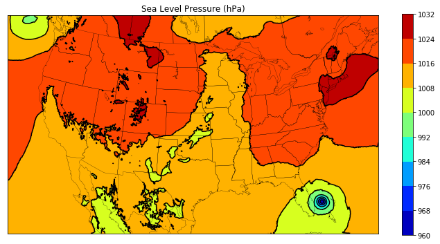
Plotting a Two-Dimensional Field
from netCDF4 import Dataset
import matplotlib.pyplot as plt
from matplotlib.cm import get_cmap
from mpl_toolkits.basemap import Basemap

from wrf import to_np, getvar, smooth2d, get_basemap, latlon_coords

# Open the NetCDF file
ncfile = Dataset("wrfout_d01_2016-10-07_00_00_00")

# Get the sea level pressure
slp = getvar(ncfile, "slp")

# Smooth the sea level pressure since it tends to be noisy near the
# mountains
smooth_slp = smooth2d(slp, 3, cenweight=4)

# Get the latitude and longitude points
lats, lons = latlon_coords(slp)

# Get the basemap object
bm = get_basemap(slp)

# Create a figure
fig = plt.figure(figsize=(12,9))

# Add geographic outlines
bm.drawcoastlines(linewidth=0.25)
bm.drawstates(linewidth=0.25)
bm.drawcountries(linewidth=0.25)

# Convert the lats and lons to x and y.  Make sure you convert the lats and
# lons to numpy arrays via to_np, or basemap crashes with an undefined
# RuntimeError.
x, y = bm(to_np(lons), to_np(lats))

# Draw the contours and filled contours
bm.contour(x, y, to_np(smooth_slp), 10, colors="black")
bm.contourf(x, y, to_np(smooth_slp), 10, cmap=get_cmap("jet"))

# Add a color bar
plt.colorbar(shrink=.62)

plt.title("Sea Level Pressure (hPa)")

plt.show()
Horizontal Interpolation to a Pressure Level
from netCDF4 import Dataset
import numpy as np
import matplotlib.pyplot as plt
from matplotlib.cm import get_cmap

from wrf import getvar, interplevel, to_np, get_basemap, latlon_coords

# Open the NetCDF file
ncfile = Dataset("wrfout_d01_2016-10-07_00_00_00")

# Extract the pressure, geopotential height, and wind variables
p = getvar(ncfile, "pressure")
z = getvar(ncfile, "z", units="dm")
ua = getvar(ncfile, "ua", units="kt")
va = getvar(ncfile, "va", units="kt")
wspd = getvar(ncfile, "wspd_wdir", units="kts")[0,:]

# Interpolate geopotential height, u, and v winds to 500 hPa
ht_500 = interplevel(z, p, 500)
u_500 = interplevel(ua, p, 500)
v_500 = interplevel(va, p, 500)
wspd_500 = interplevel(wspd, p, 500)

# Get the lat/lon coordinates
lats, lons = latlon_coords(ht_500)

# Get the basemap object
bm = get_basemap(ht_500)

# Create the figure
fig = plt.figure(figsize=(12,9))
ax = plt.axes()

# Convert the lat/lon coordinates to x/y coordinates in the projection space
x, y = bm(to_np(lons), to_np(lats))

# Add the 500 hPa geopotential height contours
levels = np.arange(520., 580., 6.)
contours = bm.contour(x, y, to_np(ht_500), levels=levels, colors="black")
plt.clabel(contours, inline=1, fontsize=10, fmt="%i")

# Add the wind speed contours
levels = [25, 30, 35, 40, 50, 60, 70, 80, 90, 100, 110, 120]
wspd_contours = bm.contourf(x, y, to_np(wspd_500), levels=levels,
                            cmap=get_cmap("rainbow"))
plt.colorbar(wspd_contours, ax=ax, orientation="horizontal", pad=.05)

# Add the geographic boundaries
bm.drawcoastlines(linewidth=0.25)
bm.drawstates(linewidth=0.25)
bm.drawcountries(linewidth=0.25)

# Add the 500 hPa wind barbs, only plotting every 125th data point.
bm.barbs(x[::125,::125], y[::125,::125], to_np(u_500[::125, ::125]),
         to_np(v_500[::125, ::125]), length=6)

plt.title("500 MB Height (dm), Wind Speed (kt), Barbs (kt)")

plt.show()
Panel Plots from the Front Page
This lengthy example shows how to make the panel plots on the first page of the documentation. For a simpler example of how to make a cross section plot, see Vertical Cross Section.
import numpy as np
import matplotlib.pyplot as plt
from matplotlib.cm import get_cmap
from netCDF4 import Dataset

from wrf import (getvar, to_np, vertcross, smooth2d, CoordPair,
                 get_basemap, latlon_coords)

# Open the NetCDF file
ncfile = Dataset("wrfout_d01_2016-10-07_00_00_00")

# Get the WRF variables
slp = getvar(ncfile, "slp")
smooth_slp = smooth2d(slp, 3)
ctt = getvar(ncfile, "ctt")
z = getvar(ncfile, "z")
dbz = getvar(ncfile, "dbz")
Z = 10**(dbz/10.)
wspd =  getvar(ncfile, "wspd_wdir", units="kt")[0,:]

# Set the start point and end point for the cross section
start_point = CoordPair(lat=26.76, lon=-80.0)
end_point = CoordPair(lat=26.76, lon=-77.8)

# Compute the vertical cross-section interpolation.  Also, include the
# lat/lon points along the cross-section in the metadata by setting latlon
# to True.
z_cross = vertcross(Z, z, wrfin=ncfile, start_point=start_point,
                    end_point=end_point, latlon=True, meta=True)
wspd_cross = vertcross(wspd, z, wrfin=ncfile, start_point=start_point,
                       end_point=end_point, latlon=True, meta=True)
dbz_cross = 10.0 * np.log10(z_cross)

# Get the latitude and longitude points
lats, lons = latlon_coords(slp)

# Create the figure that will have 3 subplots
fig = plt.figure(figsize=(12,9))
ax_ctt = fig.add_subplot(1,2,1)
ax_wspd = fig.add_subplot(2,2,2)
ax_dbz = fig.add_subplot(2,2,4)

# Get the basemap object
bm = get_basemap(slp)

# Convert the lat/lon points in to x/y points in the projection space
x, y = bm(to_np(lons), to_np(lats))

# Make the pressure contours
contour_levels = [960, 965, 970, 975, 980, 990]
c1 = bm.contour(x, y, to_np(smooth_slp), levels=contour_levels,
                colors="white", zorder=3, linewidths=1.0, ax=ax_ctt)

# Create the filled cloud top temperature contours
contour_levels = [-80.0, -70.0, -60, -50, -40, -30, -20, -10, 0, 10]
ctt_contours = bm.contourf(x, y, to_np(ctt), contour_levels,
                           cmap=get_cmap("Greys"), zorder=2, ax=ax_ctt)

point_x, point_y = bm([start_point.lon, end_point.lon],
                      [start_point.lat, end_point.lat])
bm.plot([point_x[0], point_x[1]], [point_y[0], point_y[1]], color="yellow",
        marker="o", zorder=3, ax=ax_ctt)

# Create the color bar for cloud top temperature
cb_ctt = fig.colorbar(ctt_contours, ax=ax_ctt, shrink=.60)
cb_ctt.ax.tick_params(labelsize=5)

# Draw the oceans, land, and states
bm.drawcoastlines(linewidth=0.25, ax=ax_ctt)
bm.drawstates(linewidth=0.25, ax=ax_ctt)
bm.drawcountries(linewidth=0.25, ax=ax_ctt)
bm.fillcontinents(color=np.array([ 0.9375 , 0.9375 , 0.859375]),
                                 ax=ax_ctt,
                                 lake_color=np.array([0.59375 ,
                                                      0.71484375,
                                                      0.8828125 ]))
bm.drawmapboundary(fill_color=np.array([ 0.59375 , 0.71484375, 0.8828125 ]),
                   ax=ax_ctt)

# Draw Parallels
parallels = np.arange(np.amin(lats), 30., 2.5)
bm.drawparallels(parallels, ax=ax_ctt, color="white")

merids = np.arange(-85.0, -72.0, 2.5)
bm.drawmeridians(merids, ax=ax_ctt, color="white")

# Crop the image to the hurricane region
x_start, y_start = bm(-85.0, np.amin(lats))
x_end, y_end = bm(-72.0, 30.0)

ax_ctt.set_xlim([x_start, x_end])
ax_ctt.set_ylim([y_start, y_end])

# Make the contour plot for wspd
wspd_contours = ax_wspd.contourf(to_np(wspd_cross), cmap=get_cmap("jet"))
# Add the color bar
cb_wspd = fig.colorbar(wspd_contours, ax=ax_wspd)
cb_wspd.ax.tick_params(labelsize=5)

# Make the contour plot for dbz
levels = [5 + 5*n for n in range(15)]
dbz_contours = ax_dbz.contourf(to_np(dbz_cross), levels=levels,
                               cmap=get_cmap("jet"))
cb_dbz = fig.colorbar(dbz_contours, ax=ax_dbz)
cb_dbz.ax.tick_params(labelsize=5)

# Set the x-ticks to use latitude and longitude labels.
coord_pairs = to_np(dbz_cross.coords["xy_loc"])
x_ticks = np.arange(coord_pairs.shape[0])
x_labels = [pair.latlon_str() for pair in to_np(coord_pairs)]
ax_wspd.set_xticks(x_ticks[::20])
ax_wspd.set_xticklabels([], rotation=45)
ax_dbz.set_xticks(x_ticks[::20])
ax_dbz.set_xticklabels(x_labels[::20], rotation=45, fontsize=4)

# Set the y-ticks to be height.
vert_vals = to_np(dbz_cross.coords["vertical"])
v_ticks = np.arange(vert_vals.shape[0])
ax_wspd.set_yticks(v_ticks[::20])
ax_wspd.set_yticklabels(vert_vals[::20], fontsize=4)
ax_dbz.set_yticks(v_ticks[::20])
ax_dbz.set_yticklabels(vert_vals[::20], fontsize=4)

# Set the x-axis and  y-axis labels
ax_dbz.set_xlabel("Latitude, Longitude", fontsize=5)
ax_wspd.set_ylabel("Height (m)", fontsize=5)
ax_dbz.set_ylabel("Height (m)", fontsize=5)

# Add titles
ax_ctt.set_title("Cloud Top Temperature (degC)", {"fontsize" : 7})
ax_wspd.set_title("Cross-Section of Wind Speed (kt)", {"fontsize" : 7})
ax_dbz.set_title("Cross-Section of Reflectivity (dBZ)", {"fontsize" : 7})

plt.show()
Vertical Cross Section
Vertical cross sections require no mapping software package and can be plotted using the standard matplotlib API.

import numpy as np
import matplotlib.pyplot as plt
from matplotlib.cm import get_cmap
import cartopy.crs as crs
from cartopy.feature import NaturalEarthFeature
from netCDF4 import Dataset

from wrf import to_np, getvar, CoordPair, vertcross

# Open the NetCDF file
filename = "wrfout_d01_2016-10-07_00_00_00"
ncfile = Dataset(filename)

# Extract the model height and wind speed
z = getvar(ncfile, "z")
wspd =  getvar(ncfile, "uvmet_wspd_wdir", units="kt")[0,:]

# Create the start point and end point for the cross section
start_point = CoordPair(lat=26.76, lon=-80.0)
end_point = CoordPair(lat=26.76, lon=-77.8)

# Compute the vertical cross-section interpolation.  Also, include the
# lat/lon points along the cross-section.
wspd_cross = vertcross(wspd, z, wrfin=ncfile, start_point=start_point,
                       end_point=end_point, latlon=True, meta=True)

# Create the figure
fig = plt.figure(figsize=(12,6))
ax = plt.axes()

# Make the contour plot
wspd_contours = ax.contourf(to_np(wspd_cross), cmap=get_cmap("jet"))

# Add the color bar
plt.colorbar(wspd_contours, ax=ax)

# Set the x-ticks to use latitude and longitude labels.
coord_pairs = to_np(wspd_cross.coords["xy_loc"])
x_ticks = np.arange(coord_pairs.shape[0])
x_labels = [pair.latlon_str(fmt="{:.2f}, {:.2f}")
            for pair in to_np(coord_pairs)]
ax.set_xticks(x_ticks[::20])
ax.set_xticklabels(x_labels[::20], rotation=45, fontsize=8)

# Set the y-ticks to be height.
vert_vals = to_np(wspd_cross.coords["vertical"])
v_ticks = np.arange(vert_vals.shape[0])
ax.set_yticks(v_ticks[::20])
ax.set_yticklabels(vert_vals[::20], fontsize=8)

# Set the x-axis and  y-axis labels
ax.set_xlabel("Latitude, Longitude", fontsize=12)
ax.set_ylabel("Height (m)", fontsize=12)

plt.title("Vertical Cross Section of Wind Speed (kt)")

plt.show()
Cross Section with Mountains
The example below shows how to make a cross section with the mountainous terrain filled.

import numpy as np
from matplotlib import pyplot
from matplotlib.cm import get_cmap
from matplotlib.colors import from_levels_and_colors
from cartopy import crs
from cartopy.feature import NaturalEarthFeature, COLORS
from netCDF4 import Dataset
from wrf import (getvar, to_np, get_cartopy, latlon_coords, vertcross,
                 cartopy_xlim, cartopy_ylim, interpline, CoordPair)

wrf_file = Dataset("wrfout_d01_2010-06-04_00:00:00")

# Define the cross section start and end points
cross_start = CoordPair(lat=43.5, lon=-116.5)
cross_end = CoordPair(lat=43.5, lon=-114)

# Get the WRF variables
ht = getvar(wrf_file, "z", timeidx=-1)
ter = getvar(wrf_file, "ter", timeidx=-1)
dbz = getvar(wrf_file, "dbz", timeidx=-1)
max_dbz = getvar(wrf_file, "mdbz", timeidx=-1)
Z = 10**(dbz/10.) # Use linear Z for interpolation

# Compute the vertical cross-section interpolation.  Also, include the
# lat/lon points along the cross-section in the metadata by setting latlon
# to True.
z_cross = vertcross(Z, ht, wrfin=wrf_file,
                    start_point=cross_start,
                    end_point=cross_end,
                    latlon=True, meta=True)

# Convert back to dBz after interpolation
dbz_cross = 10.0 * np.log10(z_cross)

# Add back the attributes that xarray dropped from the operations above
dbz_cross.attrs.update(z_cross.attrs)
dbz_cross.attrs["description"] = "radar reflectivity cross section"
dbz_cross.attrs["units"] = "dBZ"

# To remove the slight gap between the dbz contours and terrain due to the
# contouring of gridded data, a new vertical grid spacing, and model grid
# staggering, fill in the lower grid cells with the first non-missing value
# for each column.

# Make a copy of the z cross data. Let's use regular numpy arrays for this.
dbz_cross_filled = np.ma.copy(to_np(dbz_cross))

# For each cross section column, find the first index with non-missing
# values and copy these to the missing elements below.
for i in range(dbz_cross_filled.shape[-1]):
    column_vals = dbz_cross_filled[:,i]
    # Let's find the lowest index that isn't filled. The nonzero function
    # finds all unmasked values greater than 0. Since 0 is a valid value
    # for dBZ, let's change that threshold to be -200 dBZ instead.
    first_idx = int(np.transpose((column_vals > -200).nonzero())[0])
    dbz_cross_filled[0:first_idx, i] = dbz_cross_filled[first_idx, i]

# Get the terrain heights along the cross section line
ter_line = interpline(ter, wrfin=wrf_file, start_point=cross_start,
                      end_point=cross_end)

# Get the lat/lon points
lats, lons = latlon_coords(dbz)

# Get the cartopy projection object
cart_proj = get_cartopy(dbz)

# Create the figure
fig = pyplot.figure(figsize=(8,6))
ax_cross = pyplot.axes()

dbz_levels = np.arange(5., 75., 5.)

# Create the color table found on NWS pages.
dbz_rgb = np.array([[4,233,231],
                    [1,159,244], [3,0,244],
                    [2,253,2], [1,197,1],
                    [0,142,0], [253,248,2],
                    [229,188,0], [253,149,0],
                    [253,0,0], [212,0,0],
                    [188,0,0],[248,0,253],
                    [152,84,198]], np.float32) / 255.0

dbz_map, dbz_norm = from_levels_and_colors(dbz_levels, dbz_rgb,
                                           extend="max")

# Make the cross section plot for dbz
dbz_levels = np.arange(5.,75.,5.)
xs = np.arange(0, dbz_cross.shape[-1], 1)
ys = to_np(dbz_cross.coords["vertical"])
dbz_contours = ax_cross.contourf(xs,
                                 ys,
                                 to_np(dbz_cross_filled),
                                 levels=dbz_levels,
                                 cmap=dbz_map,
                                 norm=dbz_norm,
                                 extend="max")
# Add the color bar
cb_dbz = fig.colorbar(dbz_contours, ax=ax_cross)
cb_dbz.ax.tick_params(labelsize=8)

# Fill in the mountain area
ht_fill = ax_cross.fill_between(xs, 0, to_np(ter_line),
                                facecolor="saddlebrown")

# Set the x-ticks to use latitude and longitude labels
coord_pairs = to_np(dbz_cross.coords["xy_loc"])
x_ticks = np.arange(coord_pairs.shape[0])
x_labels = [pair.latlon_str() for pair in to_np(coord_pairs)]

# Set the desired number of x ticks below
num_ticks = 5
thin = int((len(x_ticks) / num_ticks) + .5)
ax_cross.set_xticks(x_ticks[::thin])
ax_cross.set_xticklabels(x_labels[::thin], rotation=45, fontsize=8)

# Set the x-axis and  y-axis labels
ax_cross.set_xlabel("Latitude, Longitude", fontsize=12)
ax_cross.set_ylabel("Height (m)", fontsize=12)

# Add a title
ax_cross.set_title("Cross-Section of Reflectivity (dBZ)", {"fontsize" : 14})

pyplot.show()